"It’s not that I’m so smart, it’s just that I stay with problems longer." Einstein

Quadrotor Control

In general the quadrotor has two inputs: the thrust force ($u_1$) and the moment ($u_2$). $u_1$ is the sum of the thrusts at each rotor
$u_1 = \sum_{i=1}^2 F_i$ ,
while $u_2$ is proportional to the difference between the thrusts of two rotors
$u_2 = L(F_1 - F_2)$ , where $L$ is the arm length of the quadrotor.

2-D Quadrotor Control

Equation Of Motion

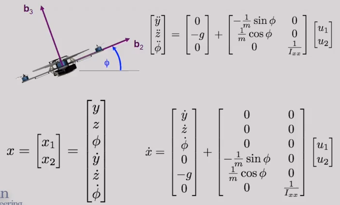
The dynamic model of the quadrotor is nonlinear. However, a PD controller is designed for a linear system. To use a linear controller for our nonlinear system, we first need to lineariye the equation of motions about a equilibrium configuration. In this case of the quadrotor, the equilibrium configuration is the hover configuration at any arbitrary position with zero angle.

Dynamics are non linear:
$\ddot{y} = -\frac{u_1}{m}\sin(\phi)$
$\ddot{z} = -g + \frac{u_1}{m}\cos(\phi)$
$\ddot{\phi} = \frac{u_2}{I_{xx}}$

Equilibrium hover configuration:
$y_0, z_0, \phi_0 = 0, u_{1,0} = mg, u_{2,0} = 0$

To linearize the dynamics, we replace all non-linear function of the state and control variables with their first order Taylor approximations at the equilibrium location.

Linearized dynamics by replacing $\sin\phi$ by $\phi$ and $\cos\phi$ by 1:
$\ddot{y} = -g\phi$
$\ddot{z} = -g + \frac{u_1}{m}$
$\ddot{\phi} = \frac{u_2}{I_{xx}}$

Trajectory Tracking

$r_T(t) = \left[\begin{matrix}y(t) \\ z(t)\end{matrix}\right]$

The desired trajectory $r(t)$ with the corresponding position, velocity and acceleration can be achieved by the commanded acceleration, calculated by the controller using:
$(\ddot{r}_T(t) - \ddot{r}_c) + \mathbf{K}_de_v + \mathbf{K}_pe_p = 0$
with $e_p = \mathbf{r}_T(t) - \mathbf{r}$
and $e_v = \ddot{\mathbf{r}}_T(t) - \ddot{\mathbf{r}}$

Nested Control Structure

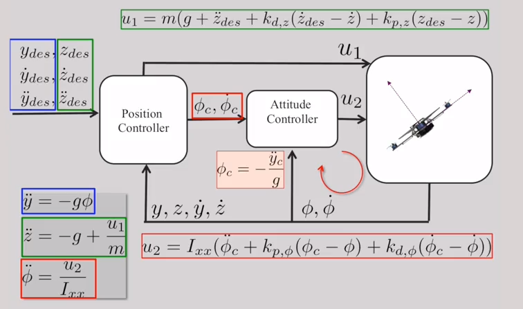
If we are following non-aggressive trajectories where the snap is small, we may approximate this as $\ddot{\phi}_c = 0$. Furthermore, we may “absorb” $\mathbf{I}_{xx}$ into the proportional and derivate gains. This gives us a new, simplified equation:
$u_2 = k_{p,\phi}(\phi_c - \phi) + k_{d,\phi}(\dot{\phi}_c - \dot{\phi})$

Control Equations

So these are the three equations we can use to drive a quadrotor that is close to the operating point and stays on the y-z-plane.

$u_1 = m(g + \ddot{z}_{des} + k_{d,z}(\dot{z}_{des} - \dot{z}) + k_{p,z}(z_{des} - z))$
$u_2 = I_{xx}(\ddot{\phi}_c + k_{d,\phi}(\dot{\phi}_c - \dot{\phi}) + k_{p,\phi}(\phi_c - \phi))$
$\phi_c = -\frac{1}{g}(\ddot{y}_{des} + k_{d,y}(\dot{y}_{des} - \dot{y}) + k_{p,y}(y_{des} - y))$

3-D Quadrotor Control

Trajectory Tracking

For the 2D quadrotor our trajectories were specified as a 2D vector $[y(t), z(t)]^T$. In the case of 3D the trajectories are specified as a 4D vector consisting of desired trajectory (position, yaw angle):

$\mathbf{r}_T(t) = \left[\begin{matrix}x(t)\\y(t)\\z(t)\\\psi(t)\end{matrix}\right]$

The desired trajectory $r(t)$ with the corresponding position, velocity and acceleration can be achieved by the commanded acceleration, calculated by the controller using:
$(\ddot{r}_T(t) - \ddot{r}_c= + \mathbf{K}_de_v + \mathbf{K}_pe_p = 0$
with $e_p = \mathbf{r}_T(t) - \mathbf{r}$
and $e_v = \ddot{\mathbf{r}}_T(t) - \ddot{\mathbf{r}}$

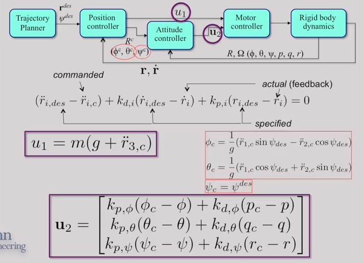
Nested Control Structure

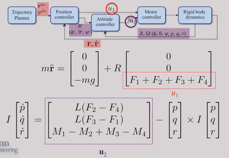
Please keep in mind that the angular velocity components in body frame are as followed:
$\left[\begin{matrix}p\\q\\r\end{matrix}\right] = \left[\begin{matrix} \cos\theta & 0 & -\cos\varphi\sin\theta \\ 0 & 1 & \sin\varphi \\ \sin\theta & 0 & \cos\varphi\cos\theta \end{matrix}\right] \left[\begin{matrix}\dot{\varphi} \\ \dot{\theta} \\ \dot{\psi} \end{matrix}\right]$

The quadrotor has two inputs: the thrust force ($u_1$) and the moment ($u_2$). $u_1$ is the sum of the thrusts at each rotor
$u_1 = \sum_{i=1}^2 F_i$
while $u_2$ is proportional to the difference between the thrusts of two rotors
$u_2 = L(F_1 - F_2)$ ($L$ is the arm lenght of the quadrotor).

Inner Loop

The inner loop corresponds to attitude control. The actual attitude and the angular velocity, or the roll, pitch and yaw angles are feed back to calculate $u_2$.

Outer Loop

The outer loop is corresponding to position control. We look mainly at the actual position vector and the yaw angle.

Control For Hovering

Let’s look at it in a special case, the hovering.
$u_1 \sim mg,\, \theta \sim 0,\, \varphi \sim 0,\, \psi \sim \psi_0$
$u_2 \sim 0,\, p \sim 0,\, q \sim 0,\, r \sim 0$

We will now linearize the dynamics at the hover configuration:

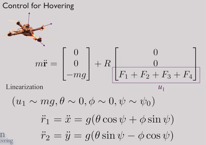
By means of these linearized equations we go further and look at the nested control structure.

Tuning PD & PID Controllers

A possible approach to tuning is to use the Zeigler-Nichols [1] method of tuning.

1. Set all gains to zero and start with the proportional gain by setting it to a rather larger value like 100 or 1000. The goal is to provoque a sustained oscillation with a rather consistend time period.
2. Once we find the $K_p$ value at which this happens, this becomes $K_u$. Also we need to find the time period of oscillations ($T_u$).
3. Calculate the other gains.
4. Repeat this steps with each group such a $y$, $z$ and $\phi$.

Planning

Time, Motion And Trajectories

General Set Up

• Start, goal positions (orientations)
• Waypoint positions (orientations)
• Smoothness criterion
  • Generally translate to minimizing rate of change of “input”
• Order of the system (n)
  • Order of the system determines the input
  • Boundary conditions on $$(n-1)^{th} order and lower derivatives
    • Third order is called yerk
    • Forth oder is called snap

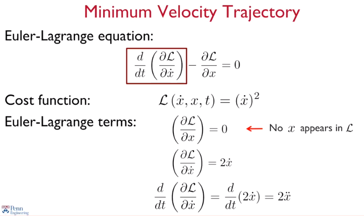
Calculus Of Variations

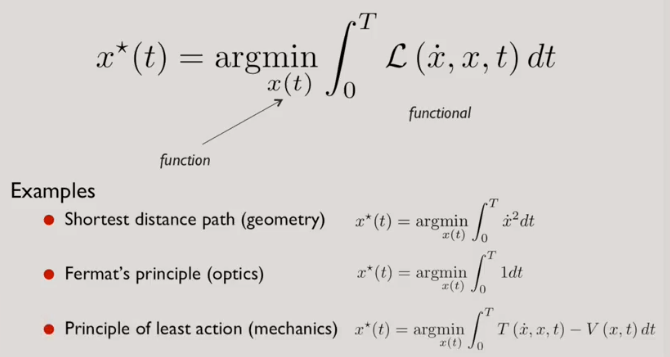
Euler Lagrange Equation

Necessary condition satisfied by the optimal function $x(t)$.

$\frac{d}{dt}\left(\frac{\partial{\mathcal{L}}}{\partial{\dot{x}}}\right) - \frac{\partial{\mathcal{L}}}{\partial{x}} = 0$

Simple Examples

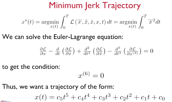
By means of the six boundary conditions at start and end positions. The position contraints looks as followed and the results becomes a linear problem:
$x(t) = c_nt^n + c_{n-1}t^{n-1} + ... + c_1t + c_0$
$x(0) = c_0 = a$
$x(T) = c_n(T)^n + ... + c_1(T) + c_0$

With differentation we get:
$\dot{x}(t) = nc_nt^n + ... + 2c_2t + c_1$

The same can be done with the acceleration and defining the corresponding boundary conditions.

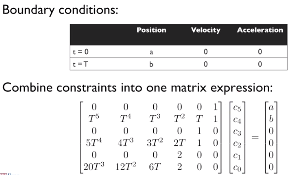
To solve this mathematical problem there are multiple possibilities. The one I’m using here is $Ax = b$
$x = A^{-1}b$
We can find a equation $x(t)$ with reflects the Minimum Jerk Trajectory.

Waypoints

In robotics it is not enough to calculate just the minimum jerk trajectory. It is necessary to calculate as well the intermediate points named waypoints. We can define piecewise continous trajectories between waypoints. Resulting in problems in to kinks of the connect pieces. Therefore we should aimed for a smooth curve, called a spline.

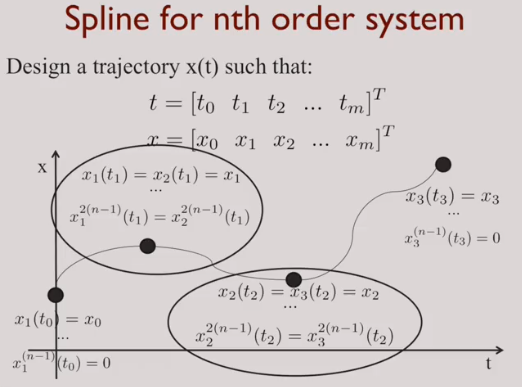
Finally, this leads us to Minimum Snap Trajectories. $x^{\star}(t) = \text{argmin}_{x(t)} \int_0^T\left(x^{(iv)}\right)^2 dt$

The position control system is a fourth order system, therefore we want trajectories that can be differentiated four times.