"I have no special talent. I am only passionately curious." Einstein

Object Localization

A Convolution Network can output a softmax layer to indicate if an object, such as a car, is present in the image. We call this Class Label. Furthermore it can also output a Bounding Box (defined by $b_x, b_y, b_h, b_w$) around the object.

Landmark Detection

For an example we’d like to find all the corners of the eyes on an image showing a face. The approach is similiar by outputting a vector with the parameter $p_{face}, l_x, l_y, ...$ with l as landmark parameter.

Object Detection

Car Detection Example

We train a ConvNet with data labeled if there is a car or not. While scanning an image we use a Sliding Window Detection by passing just a square part of the image to the ConvNet and slide it through every region of the image. Then we repeat this procedure with a different size of the sliding window.

Disadvantage Of Sliding Window Detection

Due to the huge number of the regions to check slows down the algorithm massively. Fortunately this problem of computational cost has a pretty good solution. With the help of a Convolutional Implementation we can re-use different layer’s output.

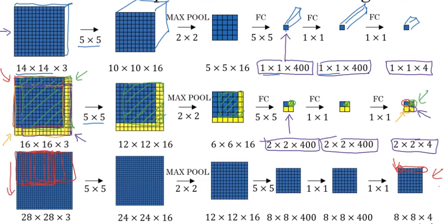
Convolutional Implementation Of Sliding Windows

Bounding Box Predictions

What if any of the BBox match with the object in the image? Is there a possibility to get the algorithm more accurate?

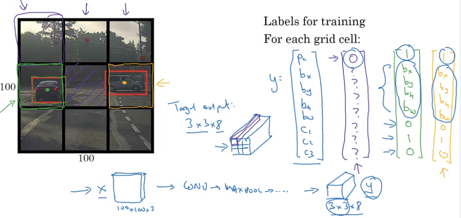
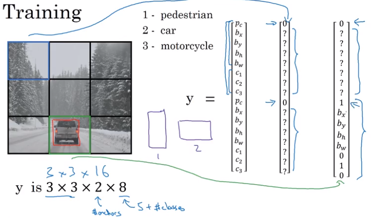
YOLO Algorithm (YOLO := You Only Look Once)

Divide the image with a grid and use the above mentioned algorithm in every grid cell.

Intersection Over Union (IoU)

It computes the intersection over two bounding boxes. $IoU = \frac{size\,of\,intersection}{size\,of\,area_{total}}$
“Correct” if $IoU \ge 0.5$

More generally, IoU is a measure of the overlap between two bounding boxes.

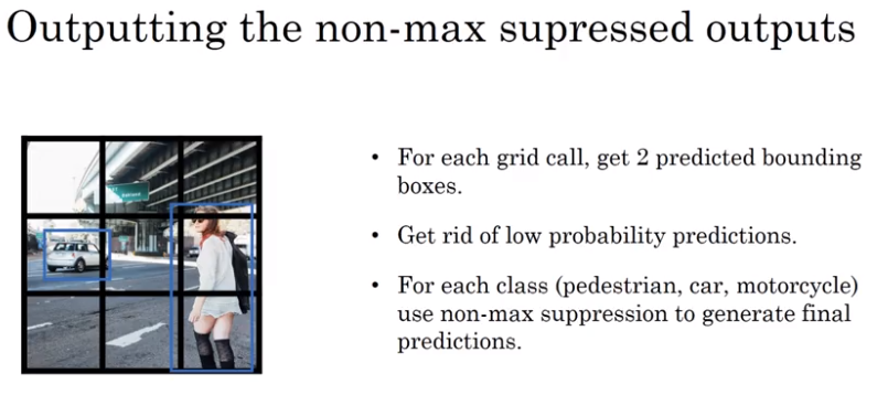
Non-max Suppression

If an object is not easily classified to belong to one single grid cell. Multiple grid cells will claim the center of object to their possession.

Cells with high IoU get darkened and the others highlighted. Then we suppress darkened cells and from the remaining we choose the cell with the highest probability.

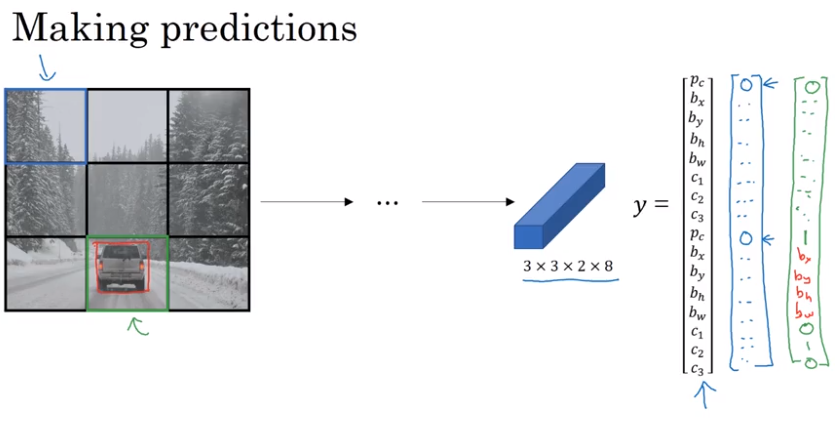
• Each output prediction is a vector $[p_c, b_x, b_y, b_h, b_w]^T$
• Discard all boxes with $p_c \le 0.6$
  • Pick the box with the largest $p_c$ and output that as a prediction
  • Discard any remaining box with $IoU \ge 0.5$ with the box ourput in the previous step

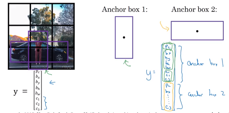
Anchor Boxes

In case of overlapping objects, the algorithm would have to choose between the object to output. This can be solved by using anchor boxes.

Algorithm

• Previously: Each object in training image is assigned to grid cell that contains that object’s midpoint.
• With two boxes: Each object in training image is assigned to grid cell that contains object’s midpoint and anchor box for the grid cell with highest IoU

More complex situations, such as three objects in the same place, have to be solved be more elaborated algorithms.

YOLO Example

Face Recognition

Verification:

• Input image, name, ID
• Output whether the input image is that of the claimed person

Recognition:

• Has a database of K persons
• Get an input image
• Output ID if the image is any of the K persons (or “not recognized”)

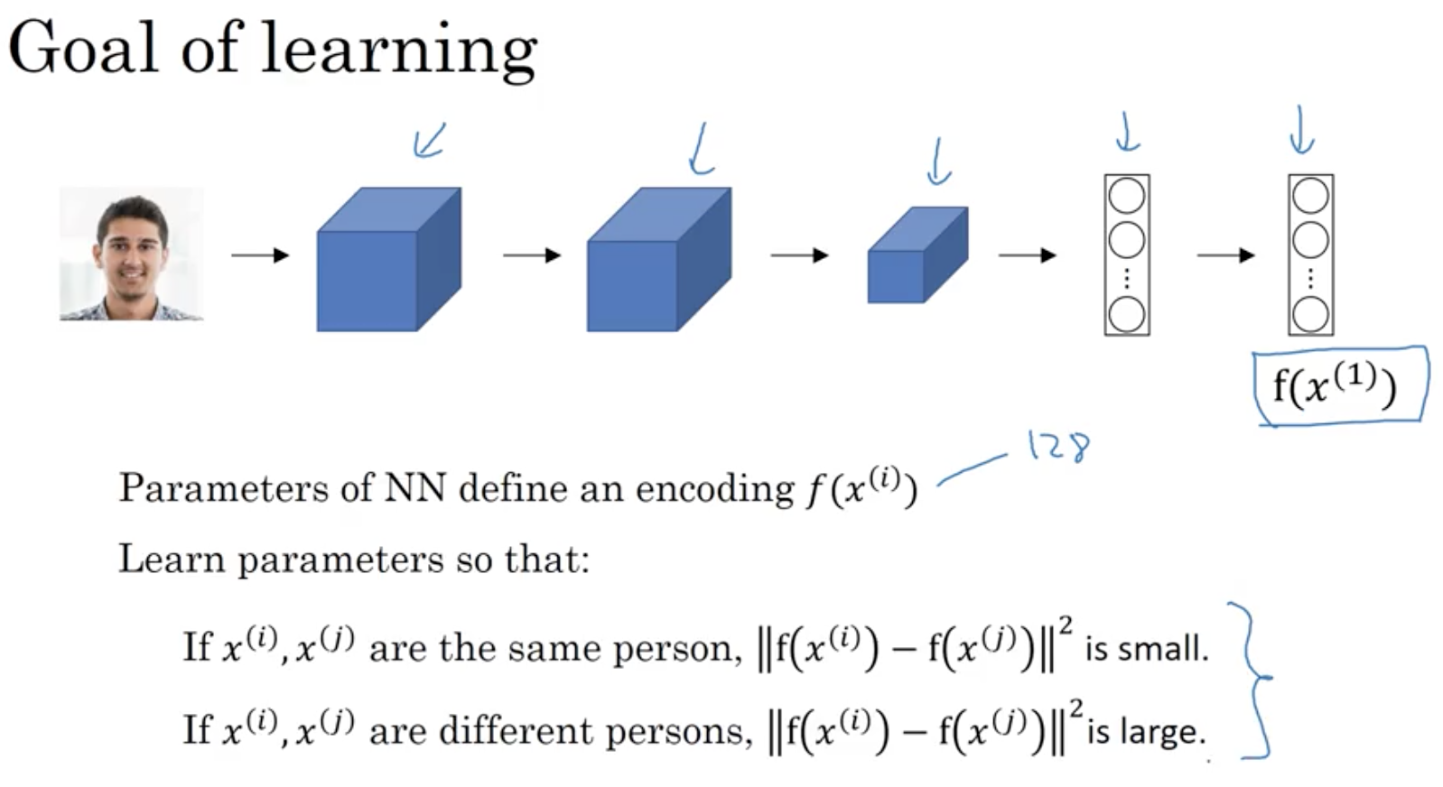
One Shot Learning Problem

Solve by getting only one example as a database. Learning from one example to recognize the person again. The algorithm has to compute a function to define the degree of difference between images and compare it to a threshold.

Siamese Network

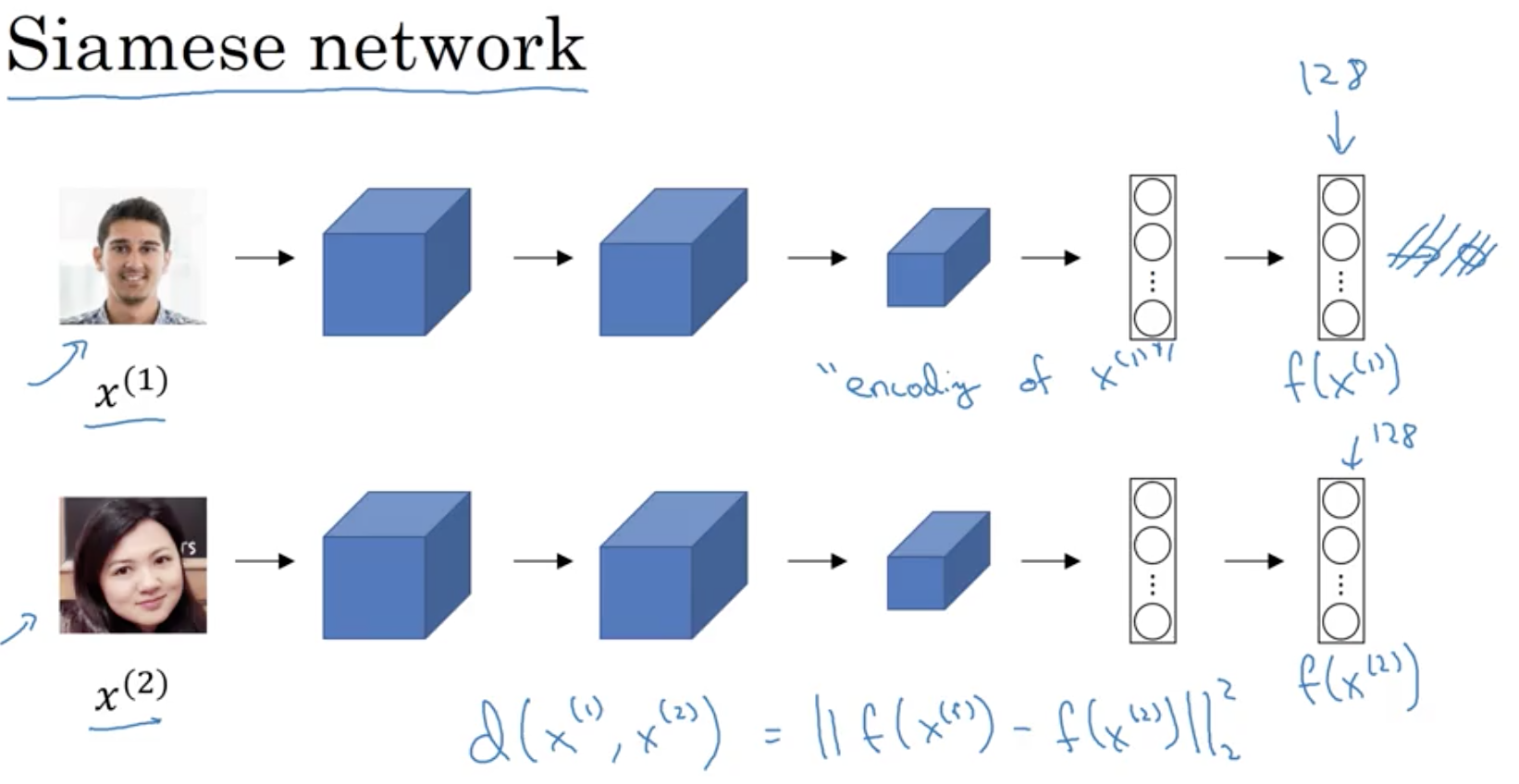
with $x^{(i)}$ and $x^{(j)}$ are different images.

Triplet Loss

The name comes from the point that we are always looking at three pictures: the anchor (A), the positive (P) and the negative (N).

We now want the difference $d(A,P) = \Vert f(A) - f(P) \Vert ^2$ and $d(A,N) = \Vert f(A) - f(N) \Vert ^2$ that
$d(A,P) \le d(A,N)$ or
$\Vert f(A) - f(P) \Vert ^2 - \Vert f(A) - f(N) \Vert ^2 + \alpha \le 0$
with $\alpha$ as a margin parameter to push the positive and the negative images further apart.

Loss Function

Given 3 images A, P, N: $\mathcal{L}(A,P,N) = max(\Vert f(A) - f(P) \Vert ^2 - \Vert f(A) - f(N) \Vert ^2 + \alpha, 0)$
Cost $J = \sum_{i=1}^m \mathcal{L}(A^{(i)}, P^{(i)}, N^{(i)})$

Most implementations also normalize the encoding vectors to have norm equal one, i.e. $\Vert f(\text{img})\Vert_2 = 1$.

# Step 1: Compute the (encoding) distance between
#  the anchor and the positive, you will need to
#  sum over axis=-1
pos_dist = tf.reduce_sum(tf.subtract(anchor, positive)**2)
# Step 2: Compute the (encoding) distance between
#  the anchor and the negative, you will need to
#  sum over axis=-1
neg_dist = tf.reduce_sum(tf.subtract(anchor, negative)**2)
# Step 3: subtract the two previous distances and
#  add alpha.
basic_loss = tf.add(tf.subtract(pos_dist, neg_dist), alpha)
# Step 4: Take the maximum of basic_loss and 0.0.
#  Sum over the training examples.
loss = tf.reduce_sum(tf.maximum(basic_loss, 0))

Choosing Triplets A, P, N

During training, if A,P,N are chosen randomly $d(A,P) + \alpha \le d(A,N)$ is easily satisfied.

Choose triplets that are “hard” to train. This is fullfilled by having $d(A,P) \approx d(A,N)$ so that the margin $\alpha$ gets to something.

Finally the cost function $J$ gets

• small for images of the same person and
• larger for images of different persons.

Face Verification & Binary Classification

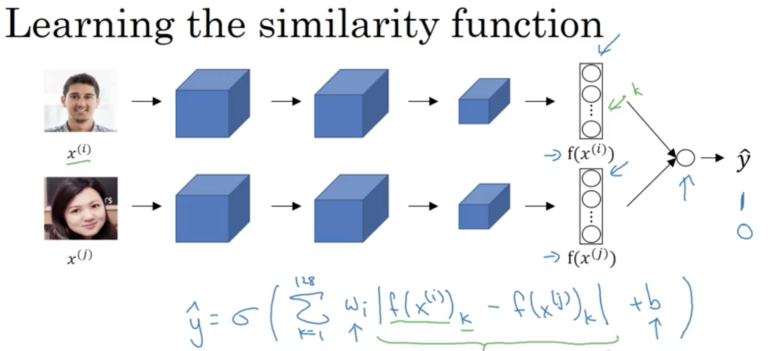
The final logistic regression will output 0 or 1 for different or same person. There different possibilities to compute the green underlined formula.

In this case we choose couplets of pictures showing the same person labeled by 1 and couplets showing two different persons labeld by 0.

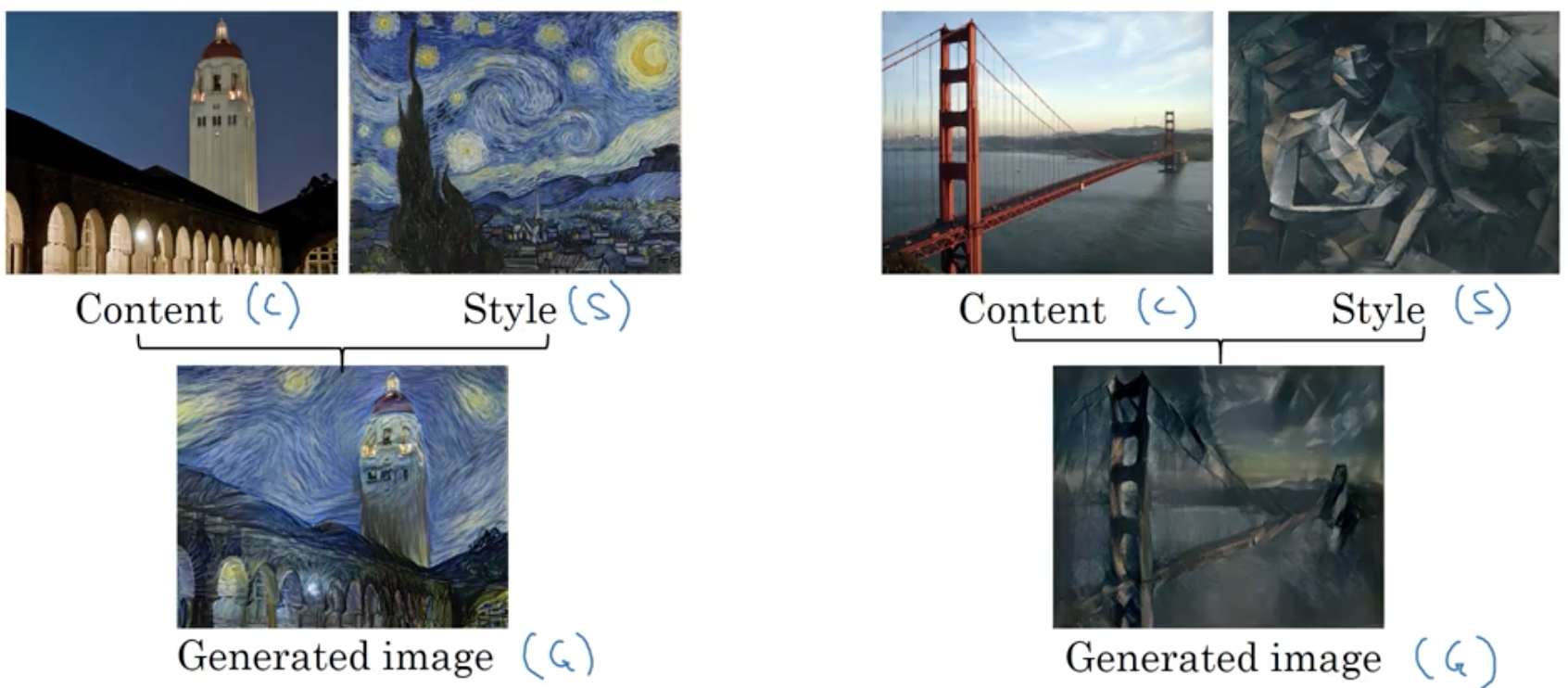
Neural Style Transfer

NST uses a previously trained convolutional network, and builds on top of that. The idea of using a network trained on a different task and applying it to a new task is called transfer learning.

Cost Function

Cost $J(G)$ is minimized by Gradient Descent.

$J(G) = \alpha J_{Content}(C, G) + \beta J_{Style}(S, G)$
with hyperparameters $\alpha$ and $\beta$.

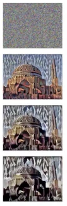
Algorithm

1. Initiate G randomly
   G: $100 \times 100 \times 3$
2. Use gradient descent to minimize $J(G)$ $G := G - \frac{\alpha}{\alpha G} J(G)$

Content Cost Function

$J(G) = \alpha\, J_{content}(C,G) + \beta\, J_{style}(S,G)$

• Say we use hidden layer l to compute content cost
• Use pre-trainend ConvNet, e.g. VGG network
• Let $a^{[l](C)}$ and $a^{[l](G)}$ be the activation of layer l on the images
• If $a^{[l](C)}$ and $a^{[l](G)}$ are similar, both images have similar content
  $J_{content}(C,G) = \frac{1}{2}\Vert a^{[l](C)}$ - $a^{[l](G)} \Vert^2$

We will define as the content cos function as:

$J_{content}(C,G) = \frac{1}{4 \times n_H \times n_W \times n_C} \sum_{\text{all entries}} (a^{(C)} - a^{(G)})^2$

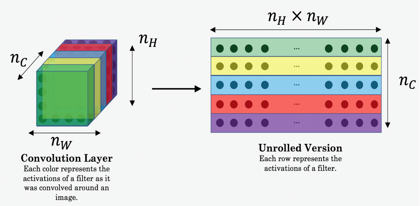
For clarity, note that $a^{(C/G)}$ are the volumes corresponding to a hidden layer’s activations. In order to compute the cost $J_{content}(C,G)$, it might be convenient to unroll these 3D volumes into a 2D matrix.

Style Cost Function

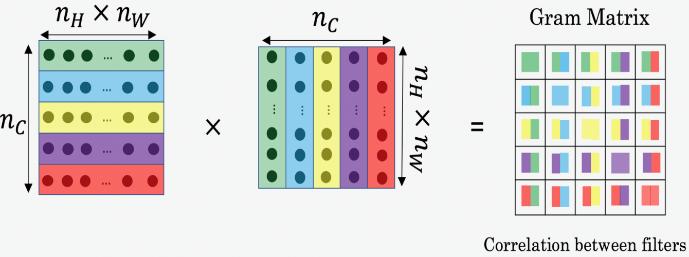
The style matrix is also called Gram Matrix. In linear algebra, the Gram matrix G of a set of vectors ($v_1, \text{...}, v_n$) is the matrix of dot products, whose entries are $G_{ij} = v_i^T \dot v_j = \text{np.dot}(v_i, v_j)$. In other words, $G_{ij}$ compares how similar $v_i$ is to $v_j$: If they are highly similar, we would expect them to have a large dot product, and thus for $G_{ij}$ to be large.

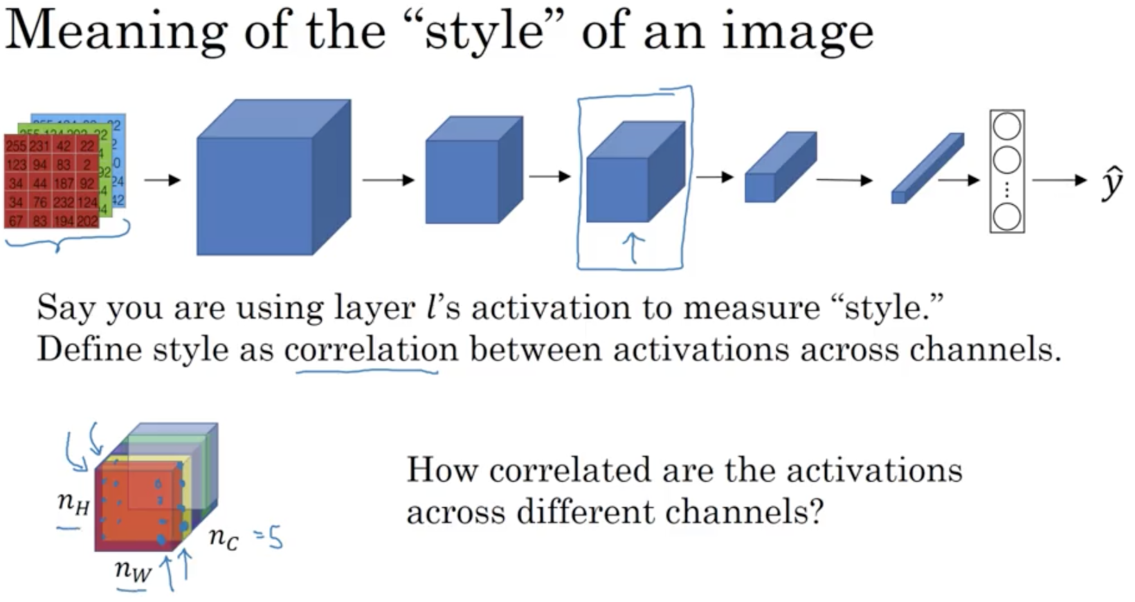
Intuition

How correlated are different channels in an image. Correlated means that if a part of the image has a certain component it appears with a second component. And therefore this two component are highly correlated. We can so measure the degree of correlation of an image and compare it with a generated image, which should have the same style.

Style Matrix

Let $a_{i,j,k}^{[l]}$ = activation at (i,j,k). $G^{[l]}$ is $n_c^{[l]} \times n_c^{[l]}$
with i,j,k as height, width and channel

$G_{kk'}^{[l]} = \sum_{i=1}^{n_H^{[l]}} \sum_{j=1}^{n_W^{[l]}} a_{ijk}^{[l]}\,a_{ijk'}^{[l]}$
with channel k to channel k’ and $k = 1, ..., n_c^{[l]}$

Correlated style results in large $G_{kk'}^{[l]}$ and vice versa.

Now we calculate the so called Gram matrix
$G_{kk'}^{[l](S)}$
$G_{kk'}^{[l](G)}$

and finally the Style cost function

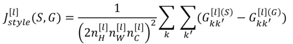
If we are using a single layer $a^{[l]}$, and the corresponding style cost for this layer is defined as:

To get better results we should summarize the cost function over multiple layers:

$J_{style}(S,G) = \sum_l \lambda^{[l]}\, J_{style}^{[l]}(S,G)$
where the values for $\lambda^{[l]}$ are style layers.

Simply said, we calculate the style cost several times, and weight them using the values from the style layers.

To create some artistic images we optimize
$J(G) = \alpha \, J_{content}(C,G) + \beta \, J_{style}(S,G)$
where $\alpha$ and $\beta$ are hyperparameters that control the relative weighting between content and style.