"A person who never made a mistake never tried anything new." Einstein
Convolutional Neural Network
In real word examples computer vision has to work on images with a size of 1000x1000x3 pixels. This becomes a huge matrix, if e.g. the first layer has 1000 knots. This results in a matrix dimension of (1000, 3M). To solve this kind of problems, we introduce convolutional neural networks.
Classical problem fields are computer vision or edge detection.
Edge Detection
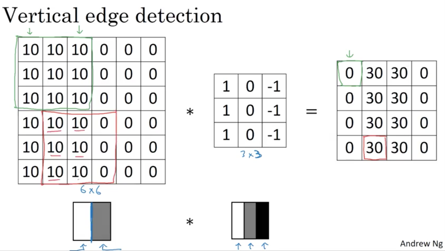
There are multiple filters developed in the past. But there is also the possibility to use Backprop to capture the values of this 3x3 filter matrix. In this sense neural networks can learn low-level features, such as edge detection.
Padding
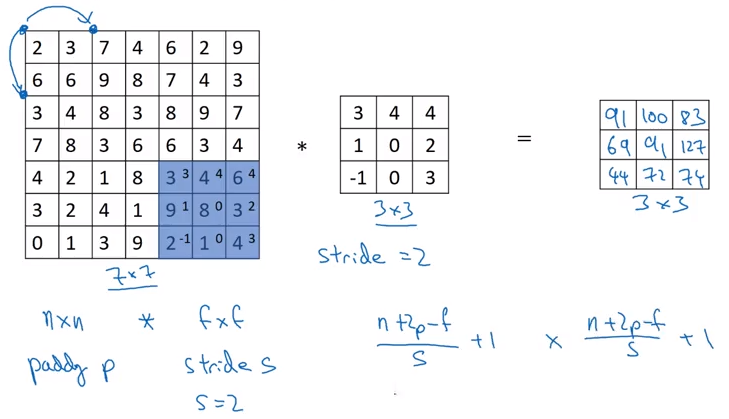
If we have a nxn image and a fxf filter, the result will be a n-f+1 x n-f+1 matrix.
To solve this shrinking output we use padding. Otherwise if every layer would shrink our image, we would loose a lot of information.
By adding an additional pixel layer around the image, we can preserve the image size. In this case the Padding p=1 and their value is zero.
Valid And Same Convolutions
- Valid: no padding
- Same: Pad so that output size is the same as the input size
To keep the input size while using a 5x5 filter, the padding would have to be p=2, meaning 2 additional surrounding pixels.
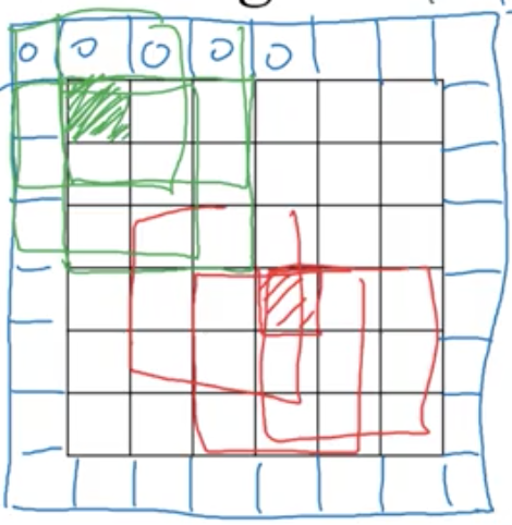
Stride Convolution
Technical Note
The convolution operation is also called cross-correletion in signal processing and math books. In this fields it’s common to flip the filter in both dimensions.
Convolutions Over Volumes
Convolutions On RGB Images
The filter will be increased in the same dimension as the image data. In this case this is 3 dimensions, for the three color channels.
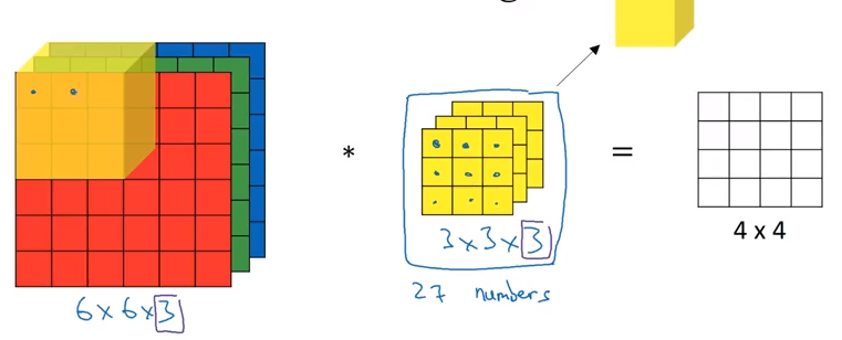
It is possible to choose by the 3D filter to switch between edge detection on single channels or multiple.
Multiple Filters
If we want to apply multiple filters such as vertical and horizontal edge detection. The results will be stacked into a multidimensional data stack with the corresponding amount of layers.
Summary
where is the amount of filters.
Convolution Layer
= filter size
= padding
= stride
= number of filters
Input:
Output:
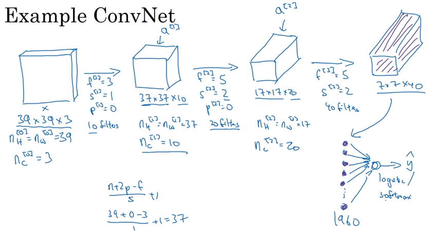
where
Each filter is:
Activations:
Weights:
Bias:
Simple Convolutional Network Example
Types Of Layer In A Convolutional Network
- Convolution
- Pooling
- Fully connected
Pooling Layer
Max Pooling
Out the filter mask, we take the max of the values. In a simple example where the input data is a 4 x 4 matrix and the filter is a 2x2 mask, we take a step of size 2. This means we have the hyperparamters f=2 and “s=2*.
In the case of a multi dimensional input layer, we perform the computation described on each of the channels indepedently.
Average Pooling
A similar approach but in the difference of taking the average of the mask covered by the filter.
Summary Of Pooling
Hyperparameters:
- f: filter size
- s: stride
- Max or Average pooling
Often we don’t use padding in case of max pooling.
In pooling there are no parameters to learn. It is just a fixed function.
Neural Network Example
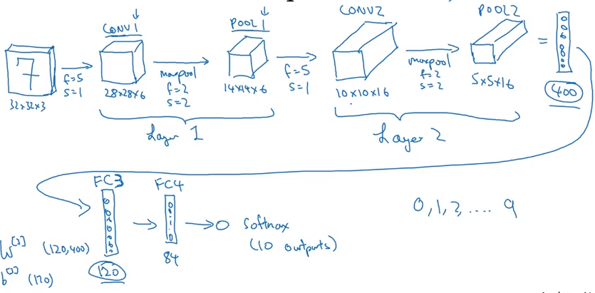
where FC3 and FC4 are Fully Connected neural networks as described in the last posts.
Putting all together we compute also a cost function and use gradient descent to optimize parameters to reduce cost J.
Why Convolutions?
- Parameter sharing: A featurer detector (edge detector) that’s useful in one part of the image is probably useful in another part of the image.
- Sparsity of connections: In each layer, ach output value depends only on asmall number of inputs.
1x1 Convolution
This is also called a Network in Network and is used to decrease and/or increase the amount of channels by maintaining the size of the input data. They are used f.ex. in inception networks.
Very Deep Convolutional Networks By Means of Residual Networks
In theory, very deep networks can represent very complex functions. But in practice, they are hard to train. Residual Networks, introduced by He et al., allow us to train much deeper networks than were previously practically feasible.
A huge barrier to training them is vanishing gradients: very deep networks often have a gradient signal that goes to zero quickly, thus making gradient descent unbearably slow.
More specifically, during gradient descent, as you backprop from the final layer back to the first layer, we are multiplying by the weight matrix on each step, and thus the gradient can decrease exponentially quickly to zero.
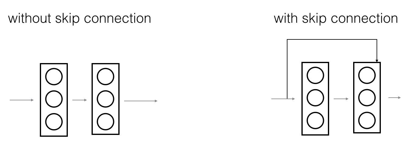
We can solve this problem by building a Residual Network. In ResNet, a shortut or a skip connection allows the gradient to be directly backpropagated to earlier layers.
After the shortcut the inputs are added to the input of the main path.
Identity Block
The identity block is the standard block usd in ResNet, and corresponds to the case where the input activation has the same dimension as the output activation .
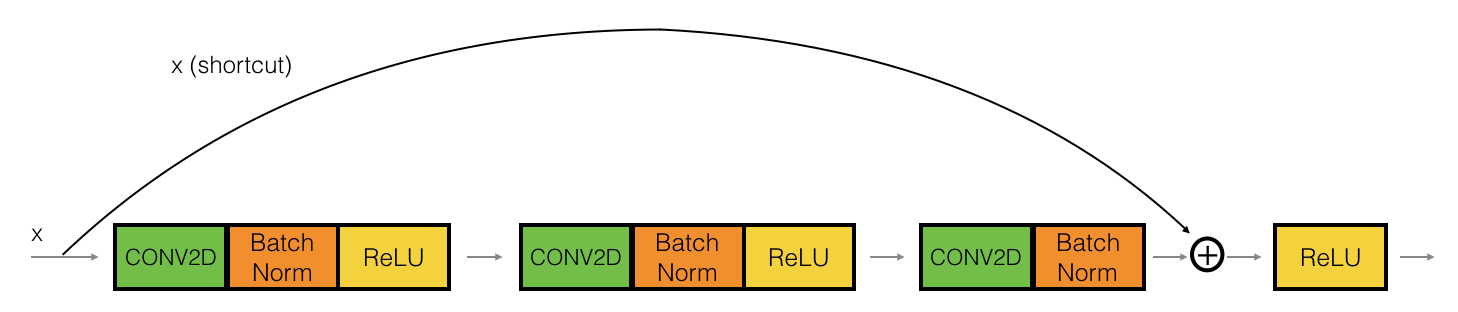
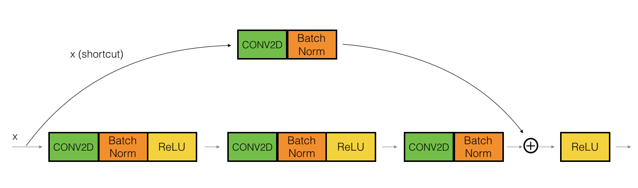
Convolutional Block
The convolutional black is the other type of block. We can use this type of block when the input and output dimensions don’t match up. The difference with the identity block is that there is a CONV2D layer in the shortcut path.