"Not everything that can be counted counts, and not everything that counts can be counted." Einstein

Unsupervised Learning

Data sets which are not labeled or group are classified by means of unsupervised learning, e.g. market segmentation or social network analysis.

One such approach is Clustering and the most common used algorithm is k-Means.

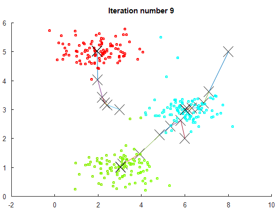
K- Means Algorithm

Input:
    *K* number of clusters
    Training set x^1, x^2, ... x^m
    drop x_0 = 1 convention

Randomly initialize N cluster centroids mu_1, mu_2, ..., mu_K
Repeat {
    for i = 1 to m
        c^(i) := index (from 1 to N) of cluster centroid closest to x^(i)
    for k = 1 to K
    	mu_k := average (mean) of points assigned to cluster *k*
}

Optimization Objective

$c^{(i)}$ = index of cluster (1,2,…,K) to which example $x^{(i)}$ is currently assigned
$\mu_k$ = cluster centroid k ($\mu_k \in \mathbb{R}^n$)
$\mu_{c^{(i)}}$ = cluster centroid of clluster to which example $x^{(i)}$ has been assigned

Optimization objective:
$J(c^{(1)},..., c^{(m)}, \mu_1,...,\mu_K) = \frac{1}{m}\sum_{i=1}^m\Vert x^{(i)} - \mu_{c^{(i)}}\Vert^2$
$min J(c^{(1)},..., c^{(m)}, \mu_1,...,\mu_K)$ regarding $c^{(i)}$ and $\mu_k$

Random Initialization of K-Means

There are few different ways, but there is one method which is most often recommended.

• Should have K < m
• Randomly pick K training examples
• Set $\mu_1, ..., \mu_K$ equal to these K examples.

Choosing The Number Of Clusters

There is not a perfect approach to choose the correct number of clusters. But there is the Elbow Method which can help.

To use the Elbow method, we have to iterate over the number of clusters and calculate the cost function for each of them. We then choose the elbow of this curve as our number of clusters.

Sometimes, we are running k-Means to get clusters to use for some later or downstream purpose. In those cases we evaluate K-Means based on a metric for how well it performs for later purpose.

Local Optima

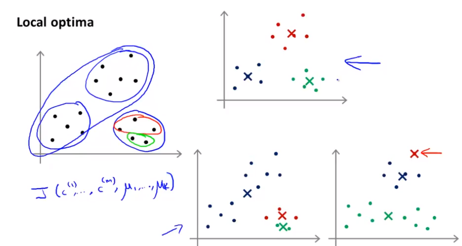
Due to various initializations the algorithm can be stucked in local optimas. To not get stuck in such a local optima, run the algorithm between 50 to 1000 times and take the parameter which create the lowest cost.

for i = 1 to 100 {
    Randomly initialize K-means
    Run K-Means. Get c^(i), ..., c^(m), mu_1, ..., mu_K.
    Compute cost function (distorsion) 
        J(c^(i), ..., c^(m), mu_1, ..., mu_K)
}

Pick clustering that gave lowest cost 
    J(c^(i), ..., c^(m), mu_1, ..., mu_K)

Principal Component Analysis

PCA helps us to reduce multi-dimensional data to 2 or 3d data. It searches for a sub-structure in our data set and our data is projected onto this structure.

PCA Problem Formulation

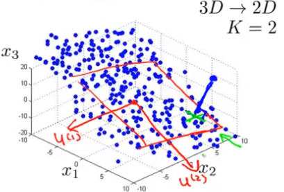
Reduce from n-dimenisional to k-dimenstional: Find k vectors $u^{(1)}, u^{(2)}, ..., u^{(k)}$ onto which to project the data, so as to minimize the projection error.

Remember: PCA is not linear regression! It projects orthogonal onto the sub-strucure!

Data Pre-Processing

We pre-process the training set by feature scaling and mean normalization: $\mu_j = \frac{1}{m}\sum_{i=1}^m x_j^{(i)}$. Then we replace each $x_j^{(i)}$ with $x_j - \mu_j$. If different features on different scales (eg. $x_1$ = size of house, $x_2$ = number of bedrooms), we should scale features to have comparable range of values.

PCA Algorithm

Our goal is to reduce from n-dimensions to k-dimensions.

For that we have to compute the covariance matrix:

$\Sigma = \frac{1}{m}\sum_{i=1}^n(x^{(i)})(x^{(i)})^T$

If the data is arranged in a matrix with rows as examples and columns as features (ex x fe), we compute the covariance matrix as such:

$\Sigma = \frac{1}{m} * X^TX$

Then we have to compute the eigenvectors of the matrix $\Sigma$ (Sigma):

[U,S,V] = svd(Sigma); 
    %svd := single value decomposition

Matrices Dimensions

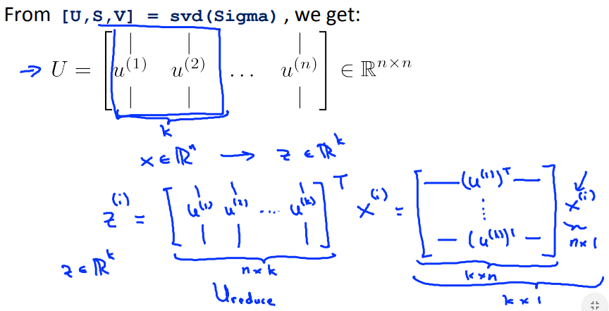
[U,S,V] = svd(Sigma); 
U_reduce = U(:,1:k);
z = U_reduce' * x;

We have to be careful regarding the dimension of data set tensors. We have to multiply each example with its features with the eigenvector to reduce it to K dimensions. This means that the above code snipped is not always correct.

Reconstruction From Compressed Representation

How do we go back from $z = U_{reduce}^T*x$? Like this: $x_{approx} = U_{reduce} * z^{(i)}$

Choosing The Number Of Principal Components

• Average squared projection error: $\frac{1}{m}\sum_{i=1}^m \Vert x^{(i)} -x_{approx}^{(i)} \Vert^2$
  
• Total variation in the data: $\frac{1}{m}\sum_{i=1}^m \Vert x^{(i)} \Vert^2$
  

Typically, we choose k in an iterative way to be smallest value so that 99% of the variance is retained:
$\frac{\frac{1}{m}\sum_{i=1}^m \Vert x^{(i)} -x_{approx}^{(i)} \Vert^2}{\frac{1}{m}\sum_{i=1}^m \Vert x^{(i)} \Vert^2} \le 0.01$ (1%)

Is most common to tell about the percentage of the retained variance as to talk about how many number of principal components have been used.

A Better Approach

[U,S,V] = svd(Sigma); 
    %svd := single value decomposition

S is a diagonal matrix and for a given k we can compute $\frac{\frac{1}{m}\sum_{i=1}^m \Vert x^{(i)} -x_{approx}^{(i)} \Vert^2}{\frac{1}{m}\sum_{i=1}^m \Vert x^{(i)} \Vert^2} \le 0.01$ with:
$1 - \frac{\sum_{i=1}^k S_{ii}}{\sum_{i=1}^n S_{ii}} \le 0.01$
Or even a bit easier:
$\frac{\sum_{i=1}^k S_{ii}}{\sum_{i=1}^n S_{ii}} \ge 0.99$

Advice for Applying PCA

Mapping $x^{(i)} \to z^{(i)}$ should be defined by running PCA only on the training set. This mapping can be applied as well to the examples $x_{cv}^{(i)}$ and $x_{test}^{(i)}$ in the cross validation and test sets.

• Compression
  • Reduce memory/disk needed to store data
  • Speed up learning algorithm
  • Choose k by % of variance retain
• Visualization
  • Chosse k equals 2 or 3

Bad Use Of PCA

Do not use PCA to prevent overfitting! This might work OK, but it isn’t a good way to address overfitting. We should use regularization instead.

Reminder on regularization: $\min_\theta \frac{1}{2m} \sum_{i=1}^m(h_\theta(x^{(i)} - y^{(i)})^2 + \frac{\lambda}{2m}\sum_{j=1}^n\theta^2$

Before implementing PCA, we should first try running whatever we want to do with the original/raw data $x^{(i)}$. Only if that doesn’t do what we want, then we implement PCA and consider using $z^{(i)}$.