"I very rarely think in words at all. A thought comes, and I may try to express in words afterwards." Einstein

Anomaly Detection

$x$ is distributed Gaussian with mean $\mu$ and variance $\sigma^2$. Also called the normal distribution.

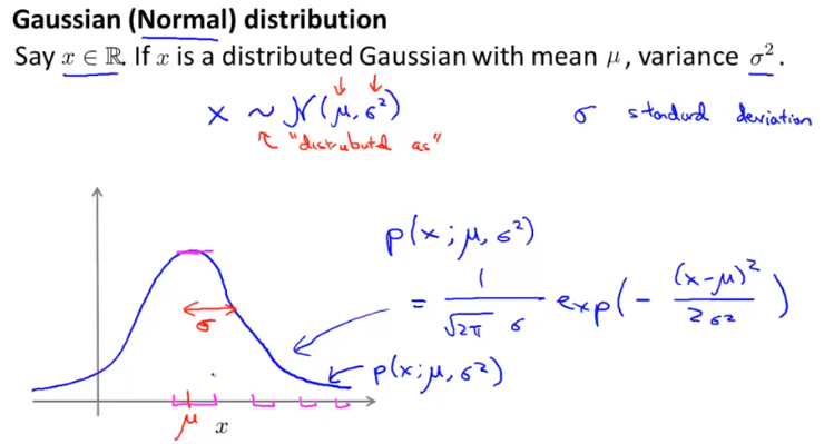
$\sigma$ is the with of the Gaussian curve and $\mu$ is where the Gaussian curve is centered.

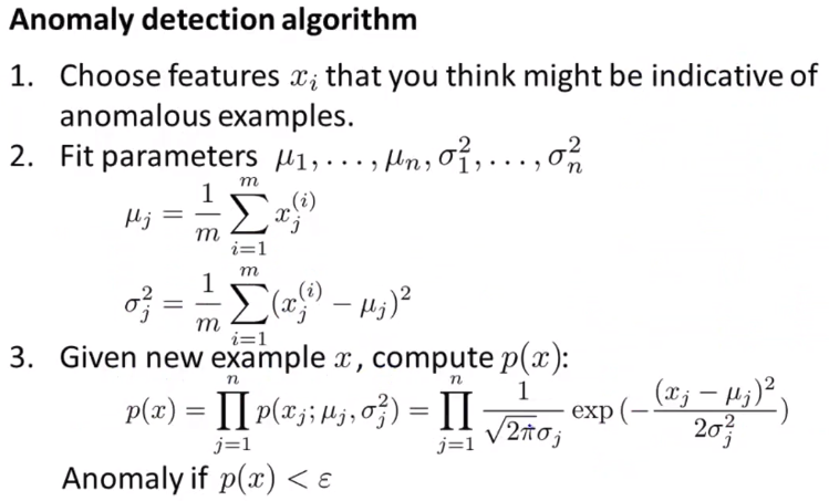
Parameter Estimation

$\mu _j= \frac{1}{m}\sum_{i=1}^m x_j^{(i)}$
$\sigma_j^2 = \frac{1}{m}\sum_{i=1}^m(x_j^{(i)} - \mu_j)^2$

This is called Maximum Likely-Hood Estimation in statistics.

Density Estimation

By using the Gaussian distribution to estimate the density of our samples.

$p(x) = p(x_1; \mu_1,\sigma_1^2)*p(x_2; \mu_3,\sigma_2^2)*...*p(x_n; \mu_n,\sigma_n^2)$
$p(x) = \prod_{j=1}^n p(x_j; \mu_j, \sigma_j^2)$

Detection Algorithm

Developing and Evaluating An Anomaly Detection System

When we develope a learning algorithm (choosing features, etc.), making a decision is much easier if we have a way of evaluating our learning algorithm.

Assume we have some labeled data of anomalous (y = 1) and non-anomalous (y = 0 if normal) examples.

We have a larger number of normal examples and some anomalous examples. We divide them as usual into train, cross-validation and test set.

Algorithm Evaluation

Possible evaluation metrics for a treshold $\epsilon$:

• True positive, false positive, false negative, true negative
• Precision/Recall
• $F_1$ Score (tells you the ground truth anomalies given a certain threshold)

$F_1 = \frac{2 \cdot prec \cdot rec}{prec + rec}$
We compute precision and recall with:
$prec = \frac{tp}{tp + fp}$
$rec = \frac{tp}{tp + fn}$
where

• tp is the number of true positives: the ground truth label says it’s an anomaly and our algorithm correctly classified it as an anomaly.
• fp is the number of false positives: the ground truth label says it’s not an anomaly, but our algorithm incorrectly classified it as an anomaly.
• fn is the number of false negatives: the ground truth label says it’s ananomaly, but our algorithm incorrectly classified it as not being anomalous.

Anomaly Detetion

• Fraud detectino
• Manufacturing (e.g. aircraft engines)
• Monitoring machines in a data center

Supervised Learing

• Email spam classification
• Weather prediction (sunny, rainy, etc.)
• Cancer classification

Choosing What Features to Use

Arrange the data in a Gaussian bell like curve. Use different transformation to make the data more gaussian, e.g. $log(x)$ or $log(x + c)$ or $x^{\frac{1}{3}}$.

% show the data as a histogram
hist(x);

Error Analysis

We want p(x) to be large for normal examples x and p(x) small for anomalous examples x.

Common Problem

The most common problem to that is, that p(x) is comparable (say, both large) for nomal and anomalous examples. A possible solution to this is trying to come up with more features to distinguish between the normal and the anomalous examples.

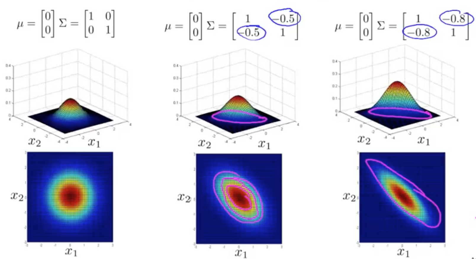
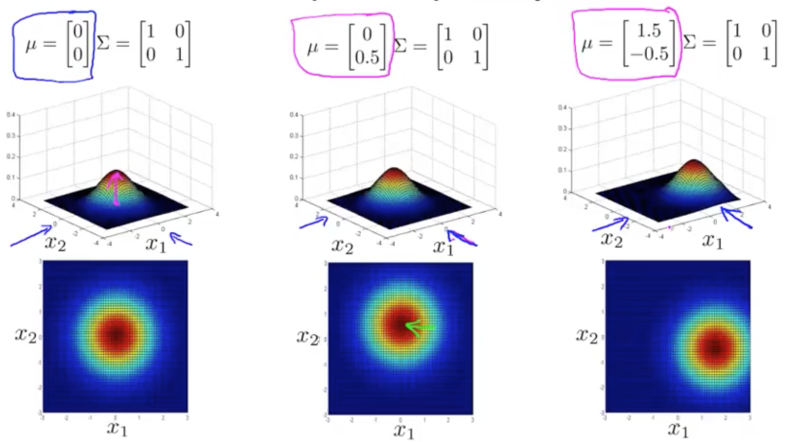
Multivariate Gaussian Distribution

$x \in \mathbb{R}^n$
We don’t model $p(x_1), p(x_2), ...$ separately, instead we model $p(x)$ all in one go. Parameters: $\mu \in \mathbb{R}^n, \Sigma \in \mathbb{R}^{n\,x\,n}$ (covariance matrix).

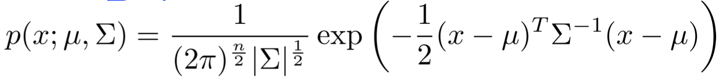
$\vert\Sigma\vert$ is the determinate and can be computed in Matlab/Octave by

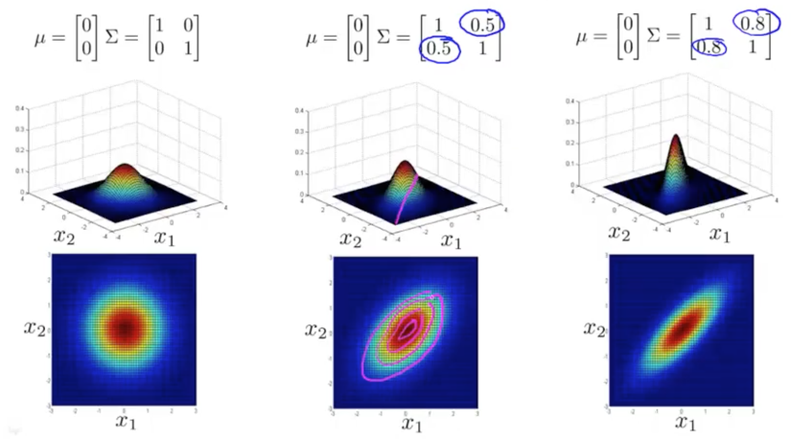
determinate = det(Sigma)

Shifting And Distorsion

Anomaly Detection With The Multivariate Gaussian

1. Fit model p(x) by setting $\mu = \frac{1}{m}\sum_{i=1}^m x^{(i)}$
   $\Sigma = \frac{1}{m}\sum_{i=1}^m (x^{(i)} - \mu)(x^{(i)} - \mu)^T$
   
2. Given a new example x, we compute p(x)

And flag an anomaly if $p(x) \lt \epsilon$.

Original Model

• Manually create features to cature anomalies where $x_1$, $x_2$ take unusual combinations of values. $x_3 = \frac{x_1}{x_2} = \frac{CPU\, load}{memory}$
  

• Computationally cheaper ( alternatively, scales better to large n).

• OK even if m (trainings set size) is small

Multivariate Gaussian

• Automatically captures correlations between features.

• Computationally more expensive.

• Must have $m \gt n$, or else $\Sigma$ is non-invertible.