"Two things are infinite: the universe and human stupidity; and I’m not sure about the universe." Einstein

A Introduction Sample

General Steps

Applied deep learning is a very empirical process. From an idea, code a solution and test it on an experiment.

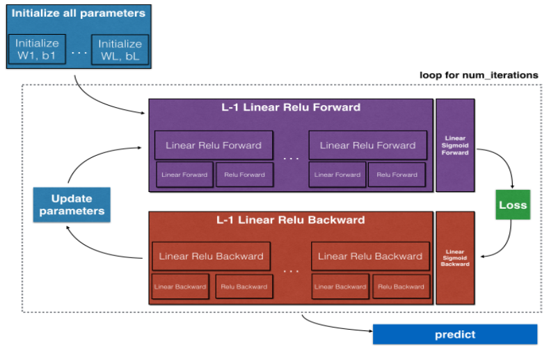The above figure gives an overview of a possible approach. This approach contains the following steps:

1. Define the neural network structure (# of input units, # of hidden units, etc)
2. Initialize the model’s parameters
3. Loop:
   • Implement forward propagation
   • Compute loss
   • Implement backward propagation to get the gradients
   • Update parameters (gradient descent)

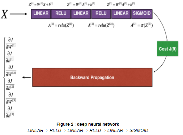
Formulas for Forward and Back Propagation

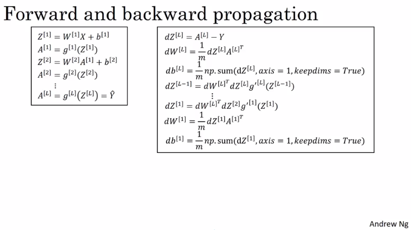
Forward Propagation

Calculate the weigths $Z^{[i]} = W^{[i]}A^{[i]} + b^{[i]}$ and the activations $A^{[i]} = g^{[i]}(Z^{[i]})$. In a neural network with n-layer, there will be a for-loop for calculating this values.

It’s completely okay to use a for-loop at this point.

Vectorized Parameters

$W^{[l]}$ is a $(n^{[l]}, n^{[l-1]}$-matrix.
$b^{[l]}$ is a $(n^{[l]}, 1)$-matrix.
$Z^{[l]}$ is a also a $(n^{[l]}, m)$-matrix. $m$ is the amount of features. The addition of b is made by means of Python’s broadcasting.

Rectified Linear Unit (ReLU)

In the context of artificial neural networks, the rectifier is an activation function defined as $f(x) = x^+ = max(0,x)$.

Intuition about Deep Representation

Example: Image input –> Edge detection –> Face subparts –> Faces

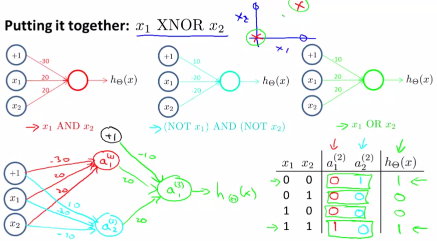
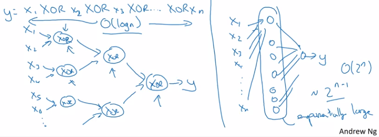
Circuit Theory and Deep Learning

Informally: There are functions you can compute with a “small” L-layer deep neural network that shallower networks require exponentially more hidden units to compute.

Gradient Descent in Neural Network

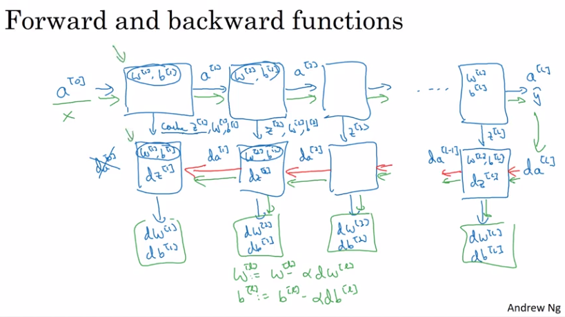
The following image shows a single step in gradient descent. It’s important to see that some values are cached.

Parameters and Hyperparameters

Parameters

$W^{[1]}$, $b^{[1]}$, $W^{[2]}$, $b^{[2]}$, $W^{[3]}$, $b^{[3]}$

Hyperparameters

• Learning rate $\alpha$
• Numbers of iterations
• Number of hidden layers
• Number of hidden units $n^{[1]}$, $n^{[2]}$, …
• Choice of activation function
• Momentum
• Minibatch size
• Regularization

Train, Dev and Test Sets

In the modern big data area the commonly used splitting of the data into 70/30 or 60/20/20 is not mostly used anymore. Instead the dev and test sets just have to be big enough, e.g. in case of 1’000’000 data samples, 10’000 examples for the dev set and 10’000 for the test set can be enough. This results into 98/1/1 or 99.5/0.4/0.1 division.

Mismatched Train/Test Distribution

Different image resolution between train and test set can lead to a mismatch. As a rule of thumb: “Make sure that dev and test sets come from the same distribution”.

Bias and Variance

Bias

Bias refers to the tendency of a measurement process to over- or under-estimate the value of a population parameter.

Variance

Variance is the expectation of the squared deviation of a random variable from its mean. Informally, it measures how far a set of (random) numbers are spread out from their average value.

Examples

From an example “Cat Classification” you have an Train Set Error of 1% and a Dev Set Error of 11%. This would mean you are performing will in train set but poorly under dev set. This looks like you have overfit the train set. So for the dev set it must be said that it has a high variance.

In a second example, we have a train set error of 15% and 16% under dev set. This means is has a high bias. It’s not even fitting the train set.

In a third example, we have a train set error of 15% and 30% under the dev set. Here you have high bias as well as high variance.

In a last example, we have a train set error of 0.5% and 1% dev set error. Here we have low bias and low variance.

Basic Recipe for Machine Learning

• High bias $\Rightarrow$ Bigger network, train longer, NN architecture
• High variance $\Rightarrow$ More data, regularization, NN architecture

Regularizing Your Neural Network

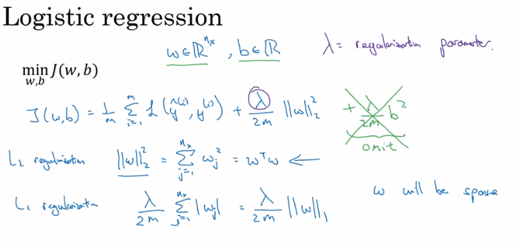
Regularize the logistic regression cost function $J(w,b)$.

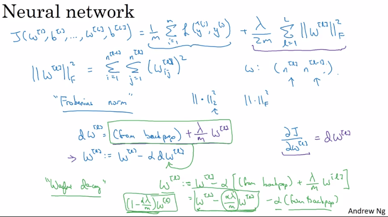
Frobenius norm used to regularize neural networks. Weight decay is also a key word in this field.

Implementation

$J(w,b) = \frac{1}{2m}\sum_{i=1}^{n_x}\mathcal{L}(\hat{y}^{[i]}, y^{[i]}) + \frac{\lambda}{2m}\sum_l^L\Vert w^{[l]}\Vert_F^2$

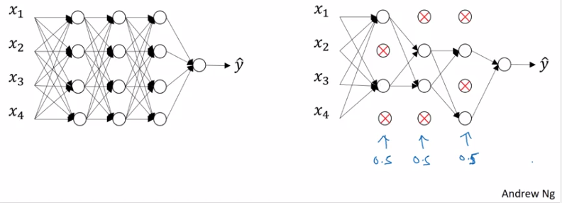
Dropout

Go through all layers of the network, and flipping a coin if the node is going to be eliminated or not.

Usage

• Use dropout only during training. Don’t use it during test time.
• Apply dropout both during forward and backward propagation.
• During training time, divide each dropout layer by keep_prob to keep the same expected value for the activations. For example, if keep_prob is 0.5, then we will on average shut down half the nodes, so the output will be scaled by 0.5 since only the remaining half are contributing to the solution. Dividing by 0.5 is equivalent to multiplying by 2. Hence, the output now has the same expected value. You can check that this works even when keep_prob is other values than 0.5.

Basic Principles Why Dropout Works

Intuition: Can’t rely on any one feature, so have to spread out weights. This shrinks the importance of single weights. Keep-Probabilities “keep_probs” can vary for different layer. Usually larger layers have a smaller probability than smaller layers. The downside is that this increases the hyper-parameters of the network. Dropout is mostly used in image recognition areas, where we always have to few data. Downside: Cost function $J$ is less defined.

Implementing Dropout

Illustrate with the layer l= 3. The keep_prob is 0.8 and d3 is the dropout matrix, with a 80% chance to be 1 and 20% to be 0 and therefore be eliminated.

Step 1: Create a random matrix if nodes be eliminated or not. $d3 = np.random.rand(a3.shape[0], a3.shape[1]) < keep\_prob$
Step 2: Eliminated the nodes in the activation layer a3. $a3 = np.multiply(a3, d3)$
Step 3: Scaling up the remaining values due to the loss by eliminating nodes. $a3 /= keep\_prob$

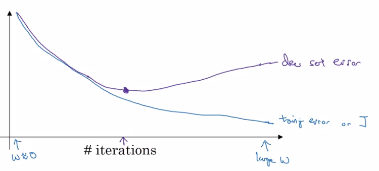
Early Stopping

Stopping learning at the best point. Downside is that it couples the optimizing and the not-overfitting tools. Relates to Orthogonalization.

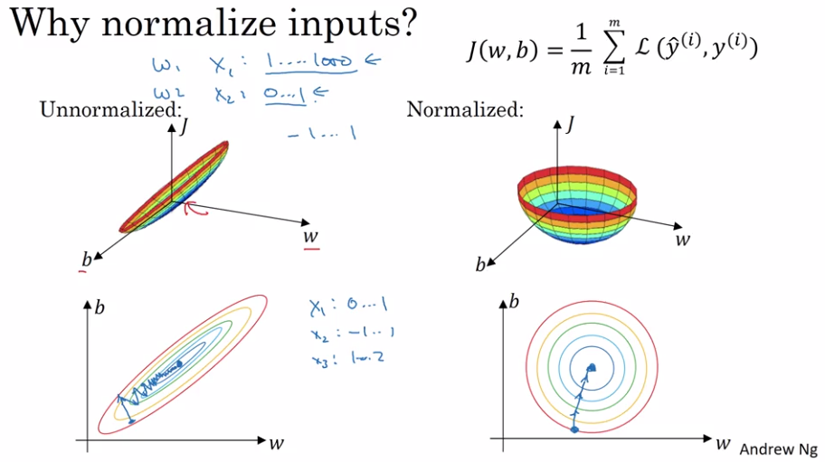
Normalizing Input Data

Weight Initialization for Deep Networks

In very deep neural networks a problem named vaninshing/exploding gradients has to be faced. One possible approach to this is a more specific initialization of the weights.

We are looking for weights that are not to larger or to small. Therefore we initialize the Matrix $W$ with values related to $$Var(w) = \frac{1}{n}.

$W^l = np.random.randn(shape) * np.sqrt(\frac{1}{n^{[l-1]}}$

Side mark: If we use a ReLU activation function we use $Var(w) = \frac{2}{n}$.

Xavier et al. showed that in case of $tan(h)$ activation function is is better to use $Var(w) = \frac{1}{n^{[n-l]}}$.

Gradient Checking

Take $W^{[1]}$, $b^{[1]}$, …, $dW^{[L]}$, $b^{[L]}$ and reshape into a big vector $\theta$.
Take $dW^{[1]}$, $db^{[1]}$, …, $dW^{[L]}$, $db^{[L]}$ and reshape into a big vector $d\theta$.

$for\, each\, i:$
$\,\,\,\,\,\,\,\,\,\,\theta_{approx}[i] = 1/2*\epsilon * ( J(\theta_1,\, \theta_2,\ ...,\, \theta_i + \epsilon) - J(\theta_1, \theta_2, ..., \theta_i - \epsilon) );$
$CheckEuclideanDist((d\theta_{approx} - d\theta) / (d\theta_{approx} + d\theta))$

Epsilon $\epsilon$ should be in the range of $10^{-7}$.

Additional Implementation Notes

• Don’t use in training - only to debug
• If algorithm fails grad check, look at components to try to identify bug
• Remember regularization
• Doesn’t work with dropout
• Run at random initialization; perhabs again after some training

Used within Back Propagation

$\frac{\partial{J}}{\partial{\theta}} = \lim_{\epsilon\to0}\frac{J(\theta + \epsilon) - J(\theta - \epsilon)}{2\epsilon}$

Relative Difference

difference $= \frac{\Vert{grad - grad_{approx}}\Vert_2}{\Vert{grad}\Vert_2 + \Vert{grad_{approx}}\Vert_2}$

Implementation Notes

$\Vert{grad - grad_{approx}}\Vert_2 = np.linalg.norm(grad - grad_{approx})$