"Do not worry about your difficulties in Mathematics. I can assure you mine are still greater." Einstein

Mini-batch Gradient Descent

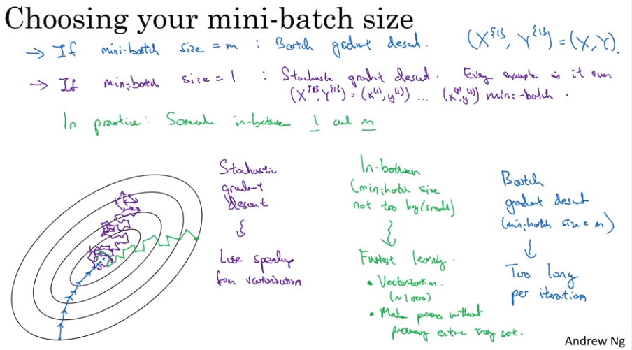
Looking back to Batch Gradient Descent, Vectorization allows us to efficiently compute on m examples. But if m is big it is still very slow because you have to train the complete training set.

Mini-batch Gradient Descent splits up the data samples into baby batches. Mini-batch t $= X^{\{t\}}$

How It Works

for $t = 1, ..., 500$
$\,\,\,\,$ Forward-Prop on $X^{\{t\}}$
$\,\,\,\,\,\,\,\, Z^{[1]} = W^{(1)}X^{\{t\}} + b^{[1]}$
$\,\,\,\,\,\,\,\, A^{[1]} = g^{[1]}(Z^{[1]})$
$\,\,\,\, ...$
$\,\,\,\,\,\,\,\, A^{[l]} = g^{[l]}(Z^{[l]})$
$\,\,\,\,$ Compute Cost $J = \frac{1}{1000}\sum_{i=0}^l\mathcal{l}(\hat{\hspace{0pt}y}^{(i)}, y^{(i)}) + \frac{\lambda}{2*1000}\sum_l\Vert{W^{[l]}}\Vert_F^2$
$\,\,\,\,$ Backprop to compute gradients cost $J^{\{t\}}$ (using ($(X^{\{t\}}, Y^{\{t\}}))$)
$\,\,\,\, W^{[l]} = W^{[l]} - \alpha\,dW^{[l]}$
$\,\,\,\, b^{[l]} = b^{[l]} - \alpha\,db^{[l]}$

Mini-batch Size

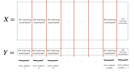
Make sure that the mini-batch fits in the CPU/GPU memory (64, 128, 256, 512).

Shuffling

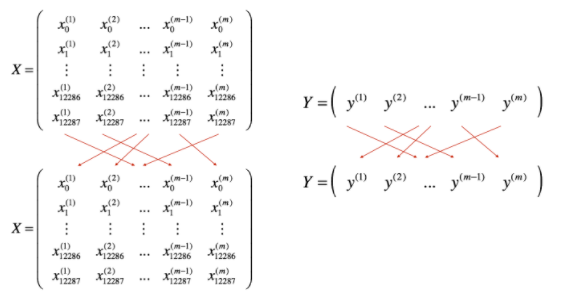
Partition

Exponentially Weighted Averages

$V_t = \beta\, V_{t-1} + (1 - \beta)\theta_t$
While $\beta \to 1$ we are averaging over larger data. $\beta$ is a hyperparameter.

How It Works

$V_t = \beta\, V_{t-1} + (1 - \beta)\theta_t$
$V_{100} = 0.1 * 0.9^0 * \theta_{100} + 0.1 * 0.9^1 * \theta_{99} + ...$
This is an exponentially decaying function and this becomes to $V_{100}$.

Implementation Notes

$Repeat$
$\,\,\,\, Get\, next\, \theta_t$
$\,\,\,\, V_{\theta} = \beta V_{\theta} + (1-\beta) \theta_t$

Bias Correction in Exponentially Weighted Average

The curve from the above equation starts very low due to the initialization of $V_0$ with 0.

$\frac{V_t}{1-\beta^t}$ is used for bias correction. But bias correction is not applied very often.

Gradient Descent With Momentum

Used to prevent diverting and/or overshooting gradient descent. The goal is to achieve a specific gradient descent faster in broader elipses and slower in narrower elipses

Average Steps

$On\, iteration\, t:$
$\,\,\,\, Compute\, dW,\, db\ on\, current\, mini batch$
$\,\,\,\, V_{dW} = \beta V_{dW} + (1-\beta)dW$
$\,\,\,\, V_{db} = \beta V_{db} + (1-\beta)db$
$\,\,\,\, W = W - \alpha V_{dW}; b = b - \alpha V_{db}$

Physical Description

Look at it as a ball is rolling down a bowl, where $V_{dW}$ and $V_{db}$ are the velocities, the derivatives the gaining acceleration and $\beta$ the friction. It is easy to imagine how the ball is rolling down.

Hyperparameters

This introduces a new hyperparameter $\beta$ to the existing $\alpha$. Normally start with $\beta = 0.9$.

RMSprop

$On\, iteration\, t:$
$\,\,\,\, Compute\, dW,\, db\ on\, current\, mini batch$
$\,\,\,\, S_{dW} = \beta S_{dW} + (1-\beta)dW^2$
$\,\,\,\, S_{db} = \beta S_{db} + (1-\beta)db^2$
$\,\,\,\, W = W - \alpha \frac{dW}{\sqrt{S_{dW}}}; b = b - \alpha \frac{db}{\sqrt{S_{db}}}$

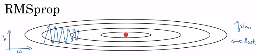
Element-wise squaring of the acceleration.

Adam Optimization Algorithm

Adam := Adaptive Moment Estimation

This is a combination of gradient descent with momentum and RMSprop.

Implementation

1. It calculates an exponentially weighted average of past gradients, and stores it in variables $v$ (before bias correction) and $v^{corrected}$ (with bias correction).
2. It calculates an exponentially weighted average of the squares of the past gradients, and stores it in variables $s$ and $s^{corrected}$.
3. It updates parameters in a direction based on combining information from “1” and “2”.

The update rule is:

$V_{dW} = 0, S_{dW} = 0, V_{db} =, S_{db} = 0$
$On\, iteration\, t:$
$\,\,\,\, Compute\, dW,\, db\ using\, current\, mini batch$
$\,\,\,\, V_{dW} = \beta_1 V_{dW} + (1-\beta_1)dW$
$\,\,\,\, V_{db} = \beta_1 V_{db} + (1-\beta_1)db$
$\,\,\,\, S_{dW} = \beta_2 S_{dW} + (1-\beta_2)dW^2$
$\,\,\,\, S_{db} = \beta_2 S_{db} + (1-\beta_2)db^2$
$\,\,\,\, V_{dW}^{corrected} = \frac{V_{dW}}{(1 - \beta_1^t)}, V_{db}^{corrected} = \frac{V_{db}}{(1 - \beta_1^t)}$
$\,\,\,\, S_{dW}^{corrected} = \frac{S_{dW}}{(1 - \beta_2^t)}, \,\,\,\, S_{db}^{corrected} = \frac{S_{db}}{(1 - \beta_2^t)}$
$\,\,\,\, W = W - \alpha \frac{V_{dW}^{corrected}}{\sqrt{S_{dW}^{corrected}} + \epsilon}, b = b - \alpha \frac{V_{db}^{corrected}}{\sqrt{S_{db}^{corrected}} + \epsilon}$

where:

• $t$ counts the number of steps taken of Adam
• $\beta_1$ and $\beta_2$ are hyperparameters that control the two exponentially weighted averages
• $\alpha$ is the learning rate
• $\epsilon$ is a very small number to avoid diving by zero

Hyperparameters Choice

$\alpha$ := needs to be tuned
$\beta_1 := 0.9$
$\beta_2 := 0.999$
$\epsilon := 10^{-8}$

Learning Rate Decay

One epoch is 1 pass through the data.

$\alpha = \frac{1}{1 + decayRate * epochNum} * \alpha_0$

$Epoch \to \alpha$
$1 \to 0.1$
$2 \to 0.067$
$3 \to 0.05$
$4 \to 0.04$

Other Methods

$\alpha = 0.95^{epochNum} * \alpha_0$
$\alpha = \frac{k}{\sqrt{epochNum}} * \alpha_0$

Problem of Local Optima

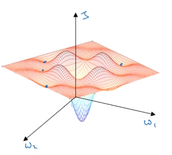
Other possiblities are sattel point, meaning it is shaped as a horse sattel and therefore zero points are no always local or global minimas.

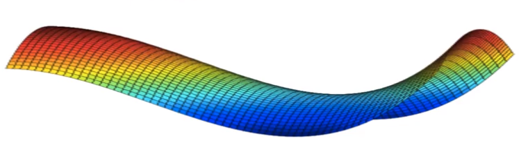
Platforms can make learning very slow and then ADAM and likewise can really help to speed up the training.

Tuning Process

• The following hyperparameters can be tuned: $\alpha$, $\beta$, #layers, #hidden units, learning rate decay, mini-batch size.
• It is better to try random values instead of using a parameter grid.
• We should use a coarse to fine sampling scheme

Appropriate Scale To Pick Hyperparameters

• Use a logarthmic scale to chose from for the learning rate $\alpha$.

Possible implementation in Python:

1
2
3
4
# Values between 0.0001 and 1
def scaleLearningRate:
   r = -4 * np.random.rand()	
   learning_rate = np.power(10, r)

In pratice, hyperparameters can be tuned by means of Pandas or Caviar. It’s good pratice to re-evaluate the parameters every month or so.

During development a model can be babysit one model. Another approach would be to train many models in parallel. The first babysitting approach is callend Panda and the second is the Caviar approach.

This mainly depends on the resources we have at hand and the size of data to be processed.

There is a another approach which not always fits the problem we are facing. It is possible to normalize the activations in a network.

Batch Normalization

Batch normalization allows to train deeper neural networks, makes the hyperparameter search more easier and the network much more robust. Usually it is used with mini-batches. Batch norm are used per first mini-batch, then second and so on.

Idea

Normalized inputs speed up learning. The question is can we normalize $a^{[2]}$ so as to train $W^{[3]}$, $b^{[3]}$ faster? This is what Batch Normalization is doing.

Implementation

Given some intermediate values in my NN $z^{(i)}, ..., z^{(m)}$
$\mu = \frac{1}{m}\sum_i z^{(i)}$
$\sigma^2 = \frac{1}{m}\sum_i(z_i - \mu)^2$
$Z_{norm}^{(i)} = \frac{z^{(i)} - \mu}{\sqrt{\sigma^2 + \epsilon}}$
$\tilde{z}^{(i)} = \gamma z_{norm}^{(i)} + \beta$

where

• $\gamma$ and $\beta$ are learnable hyperparameters of the model
• $$\gamma = \sqrt{\sigma^2 + \epsilon}$$
• $$\beta = \mu$$
• Use $\tilde{Z}^{[l](i)}$ instead of $Z^{[l](i)}$

for t = 1 ... numMiniBatches
	Compute forward prop on X_T
    	In each hidden layer, use N to replace z_l with zTilde_l
    Use back prop to compute dW_l, db_l, dBeta_l, dGamma_l
    Update the parameters 
    	W_l = W - alpha * dW_l
        beta_l = beta_l - alpha * dBeta_l
        gamma_l = gamma_l - alpha * dGamma_l    

Learning On Shifting Input Distribution

A trained NN can not be easilier applied to a shifted version of training data. This is called covariance shift.

Image an deeper NN where the later hidden layers would perfectly fit the problem, but the first few hidden layer not, we would have to shift the NN to fit the new problem. This can be done by Batch Norm.

A second effect coming from batch norm:

• Each mini-batch is scaled by the mean/veriance omputed on just that mini-batch
• This adds some noise to the values $z^{[l]}$ within that minibatch. So similar to dropout, it adds some noise to each hidden layer’s activation
• This has a slight regularization effect.

Batch Norm At Test Time

$\mu = \frac{1}{m} \sum_i z^{(i)}$
$\sigma^2 = \frac{1}{m} \sum_i (z^{(i)} - \mu)^2$
$z_{norm}^{(i)} = \frac{z^{(i)} - \mu}{\sqrt{\sigma^2 + \epsilon}}$
$\tilde{z}^{(i)} = \gamma z_{norm}^{(i)} + \beta$

The first two equation cannot be computed during test time, therefore we estimate $\mu$ and $\sigma^2$ using exponentially weigthed average (across mini-batches). Most frameworks offers an interface to create $\mu$ and $\sigma$.

Softmax Layer

The softmax layer function has the special ability to take a vector as input instead of a single value. Otherwise it is similar to the activation function.

The names come from the hard max approach where a multiclass classification results are mapped to a vector, eg. for being a result of the first class of 4:
$\begin{bmatrix} 1 \\ 0 \\ 0 \\ 0 \\ \end{bmatrix}$

Softmax is normalizing the classification values instead of the above mentioned hard coded vector.

Examples

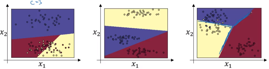
Separate the date into for example three different classes, where the softmax layer can be seen as a generaization of the logistic regression.

Training A Softmax Classifier

Softmax regression generalizes logistic regression to C classes. If $C = 2$, softmax reduces to logistic regression. We would have to compute only one output.

Lost Function

$\mathcal{L}(\tilde{y},y) = - \sum_{j=1}^{m} y_i\,log\tilde{y}_j$

Backward Propagation

$dz^{[L]} = \tilde{y} - y$