"Do not worry about your difficulties in Mathematics. I can assure you mine are still greater." Einstein

What to keep in mind regarding Calculus for Back Propagation.

Introduction

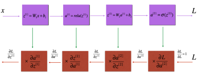
To compute derivates in Neural Networks a Computation Graph can help. It contains both a forward and a back propagation.

Back propagation contains Calculus, or more specific we have to take different Derivatives. Look at it as a computation from right to left.

Chain Rule

$u = bc \Rightarrow v = a + u \Rightarrow J = 3v$

$\frac{dJ}{dv} = 3$
$\frac{dJ}{da} = \frac{dJ}{dv} * \frac{dv}{da} = 3 * 1$
$\frac{dJ}{du} = \frac{dJ}{dv} * \frac{dv}{du} = 3 * 1$
$\frac{dJ}{db} = \frac{dJ}{du} * \frac{du}{db} = \frac{dJ}{dv} * \frac{dv}{du} * \frac{du}{db} = 3 * 1 * c$

Wording

$a_j^{[2](i)}$ := layer 2, example i, neuron j

Formulas for Forward and Back Propagation

Forward Propagation

Estimation function $Z^{[i]} = W^{[i]}X + b^{[i]}$
Sigmoid function $g^{[i]} = 1/1+e^{-z}$
Node $a^{[i]} = g^{[i]}(z^{[i]})$
Loss (error) function $\mathcal{L}(\hat{y}, y) = -(y\, log(\hat{y}) + (1-y) log(1-\hat{y}))$
Logistic Regression Cost Function $J(w,b) = 1/m * \sum_{i=1}^m \mathcal{L}(\hat{y}^{[i]}, y^{[i]}) = - 1/m * \sum_{i=1}^m y^{(i)} log(\hat{y}^{[i]}) + (1-y^{[i]}) log(1-\hat{y}^{[i]})$

Vectorized implementation

$J(w,b) = -1/m * np.sum(np.multiply(Y, np.log(A^{[L]})) + np.multiply((1 - Y),np.log(1-A^{[L]})))$

Forward Propagation with Dropout

Create matrix $D^{[i]}$ with the same dimension as the corresponding activation matrix $A^{[i]}$ and initialize it randomly. Then set all values to 0 or 1 regarding the keep probability. Then multiply the activation matrix with the dropout matrix and divide the remaining values by the keep probability.

Backward Propagation

Suppose you have already calculated the derivative $dZ{[l]} = \frac{\partial{\mathcal{L}}}{\partial{Z^{[l]}}}$, then you want to get $dW^{[l]}$, $db^{[l]}$ and $dA^{[l-1]}$.

$dW^{[l]} = \frac{\partial{\mathcal{L}}}{\partial{W^{[l]}}} = \frac{1}{m} dZ^{[l]}A^{[l-1]T}$
$db^{[l]} = \frac{\partial{\mathcal{L}}}{\partial{W^{[l]}}} = \frac{1}{m} \sum_{i=1}^{m}dZ^{[l](i)}$
$dA^{[l-1]} = \frac{\partial{\mathcal{L}}}{\partial{A^{[l-1]}}} = W^{[l]T}dZ^{[l]}$
where
$dZ^{[l-1]} = W^{[l]^T}dZ^{[l]} * g'^{[l-1]}(Z^{[l]})$
$dZ^{[L]} = A^{[L]} - Y$

Summary of gradient descent

$dz^{[2]} = a^{[2]} - y$
$dW^{[2]} = dz^{[2]}a^{[1]^T}$
$db^{[2]} = dz^{[2]}$
$dz^{[1]} = W^{[2]^T}dz^{[2]} * g'^{[1]}(z^{[1]})$
$dW^{[1]} = dz^{[1]}x^T$
$db^{[1]} = dz^{[1]}$
$dA^{[l-1]} = \frac{\partial{\mathcal{L}}}{\partial{A^{[l-1]}}} = W^{[l]^T}dZ^{[l]}$

Vectorized implementation example

$dZ^{[2]} = A^{[2]} - Y$
$dW^{[2]} = \frac{1}{m} dZ^{[2]}A^{[1]^T}$
$db^{[2]} = \frac{1}{m} np.sum(dZ^{[2]}, axis=1, keepdims=True)$
$dZ^{[1]} = W^{[2]^T}dZ^{[2]} * g'^{[1]}(Z^{[1]})$
$dW^{[1]} = \frac{1}{m} dZ^{[1]}X^T$
$db^{[1]} = \frac{1}{m} np.sum(dZ^{[1]}, axis=1, keepdims=True)$
$dA^{[l-1]} = W^{[l]^T}dZ^{[l]}$
$dA^{[l]} = -(np.divide(Y, A^{[L]}) - np.divide(1-Y, 1-A^{[L]}))$
The derivative of cost with respect to $A^{[L]}$

Calculation Problem with Zero Matrix

Initialize weights with a 2x2 zero matrix is a problem. The computed a’s will be the same. And the dW rows will also be the same. This is independent how many cycles are be computed.

Random Initialization

We should initialize the parameters randomly. The parameters are $n_x$ := n of input layer, $n_h$ := n of hidden layer and $n_y$ := n of output layer
$W^{[1]} = np.random.randn(n_h,n_x) * 0.01$
$b^{[1]} = np.zeros((n_h,1))$
$W^{[2]} = np.random.randn(n_y,n_h) * 0.01$
$b^{[2]} = np.zeros((n_y,1))$

Where does the constant 0.01 comes from? We prefer to use very small initialization values. This means we will not start at the flat parts of the curve.

Xavier or He Initialization

Xavier initialization uses the factor $\sqrt{\frac{1}{n_x}}$ instead of 0.01. And He et al. proposed the slightly adapted factor $\sqrt{\frac{2}{n_x}}$.

General Gradient Descent Rule

$\theta = \theta - \alpha\frac{\partial{J}}{\partial{\theta}}$

Update Rule For Each Parameter

$W^{[i]} = W^{[i]} - \alpha * dW^{[i]}$
$b^{[i]} = b^{[i]} - \alpha * db^{[i]}$

L2 Regularization

The standard way to avoid overfitting is called L2 regularization. It consits of appropriately modifying your cost function.
$J=-\frac{1}{m}\sum_{i=1}^m[y^{(i)}log(a^{[L](i)}) +(1-y^{(i)})log(1-a^{[L](i)})]$
to:
$J_{regularized}=-\frac{1}{m}\sum_{i=1}^m[y^{(i)}log(a^{[L](i)}) +(1-y^{(i)})log(1-a^{[L](i)})] + \frac{1}{m}\frac{\lambda}{2}\sum_l\sum_k\sum_jW_{j,k}^{[l]2}$
The first term is named cross-entropy cost and the second term L2 regularization cost.

Observations

• The value of $\lambda$ is a hyperparameter that you can tune using a dev set.
• L2 regularization makes your decision boundary smoother. If $\lambda$ is too large, it is also possible to oversmooth, resulting in a model with high bias.

Implementation Details

To calculate $\sum_k\sum_j W_{k,j}^{[l]2}$ use

1
np.sum(np.square(W1))

Backpropagation With Regularization

For each node we have to add teh regularization term’s gradient $(\frac{d}{dW}(\frac{1}{2}\frac{\lambda}{m}W^2) = \frac{\lambda}{m}W$.

Backpropagation with Dropout

Multiply the derivative $dA^{[i]}$ with the corresponding droupout matrix cached in the forward propagation. Finally divide the remaining values in the activation matrix by the keep probablity.